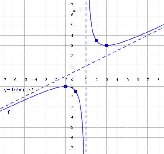
Para representar gráficamente una función, pueden seguirse los siguientes pasos:
1) Determinar el dominio
2) Hallar los puntos de corte con los ejes
3) Hallar las asíntotas de la función y estudiar la posición relativa de la gráfica con respecto a ellas
4) Estudiar la monotonía. Determinar los extremos relativos
5) Estudiar la concavidad y la convexidad
6) Realizar la representación gráfica
Ejemplo: Representa gráficamente la función \(\displaystyle f(x)=\frac{x^2+3}{2x-2}\)
1) Dominio
\(2x-2=0\iff 2x=2 \iff x=1\)
\(\hspace{1em} \boxed{\mbox{Dom}(f)=\mathbb R\setminus\{ 1\}}\)
2) Puntos de corte con los ejes
\(x=0 \hspace{1em} y=\displaystyle \frac{3}{-2}=-1.5\)
Punto de corte con el eje \(y: \hspace{1em} \boxed{(0,-1.5)}\)
\(f(x)=0 \Rightarrow x^2+3=0\longrightarrow\) No tiene solución. Por tanto, la gráfica no corta al eje \(x\)
3) Asíntota vertical:
\(\hspace{1em}\displaystyle\lim_{x\rightarrow 1^-}f(x)=\lim_{x\rightarrow 1^-} \frac{x^2+3}{2x-2}=\lim_{x\rightarrow 1^-} \frac{x^2+3}{2(x-1)} \hspace{-1.5cm} \underset{ \begin{array}{c}\uparrow \\ \small\displaystyle \lim_{x\rightarrow 1^-} (x^2+3)=4>0 \\ \small\displaystyle\lim_{x\rightarrow 1^-} (x-1)=0 \\ \small \displaystyle x-1<0 \end{array}}{=} \hspace{-1.5cm} -\infty\)
\(\hspace{1em}\displaystyle\lim_{x\rightarrow 1^+}f(x)=\lim_{x\rightarrow 1^+} \frac{x^2+3}{2x-2}=\lim_{x\rightarrow 1^+} \frac{x^2+3}{2(x-1)} \hspace{-1.5cm} \underset{ \begin{array}{c}\uparrow \\ \small\displaystyle \lim_{x\rightarrow 1^+} (x^2+3)=4>0 \\ \small\displaystyle\lim_{x\rightarrow 1^+} (x-1)=0 \\ \small \displaystyle x-1>0 \end{array}}{=} \hspace{-1.5cm} +\infty\)
La recta \(\boxed{x=1}\) es una asíntota vertical.
Asíntota oblicua:
\(\begin{array}{rl}
\mathit x^2\hspace{2em} +3 & \begin{array}{|c}2\mathit x-2\\ \hline\end{array}\\
-\mathit x^2+\mathit x \hspace{2em} & \frac 1 2\mathit x+\frac 1 2 \\
\underline{\hspace{2em} \hspace{2em}\hspace{2em} }& \\
\mathit x+3 & \\
-\mathit x +1 & \\
\underline{\hspace{2em} \hspace{2em} }& \\
4
\end{array} \hspace{2em} \hspace{2em} f(x)=\displaystyle \frac 1 2 x+\frac 1 2+\frac{4}{2x-2}\)
Como \(\displaystyle \lim_{x\rightarrow+\infty}\frac{4}{2x-2}=\displaystyle \lim_{x\rightarrow-\infty}\frac{4}{2x-2}=0\) entonces \(\boxed{y=\displaystyle \frac 1 2 x+\frac 1 2}\) es una asíntota oblicua de \(f\).
- Si \(x\rightarrow +\infty\), entonces \(\displaystyle \frac 4 {2x-2}>0\Rightarrow \) La gráfica está por encima de la asíntota oblicua
- Si \(x\rightarrow -\infty\), entonces \(\displaystyle \frac 4 {2x-2}<0\Rightarrow \) La gráfica está por debajo de la asíntota oblicua
4) Monotonía:
\(f'(x)=\displaystyle \frac{2x\cdot(2x-2)-(x^2+3)\cdot 2}{(2x-2)^2}=\)
\(=\displaystyle\frac{4x^2-4x-2x^2-6 }{(2(x-1))^2}=\)
\(=\displaystyle\frac{2x^2-4x-6 }{4(x-1)^2}=\)
\(=\displaystyle\frac{x^2-2x-3 }{2(x-1)^2}\)
\(f'(x)=0 \iff x^2-2x-3=0\)
\(x=\displaystyle \frac{2\pm\sqrt{4-4\cdot(-3)}}{2}=\frac{2\pm\sqrt{16}}2=\begin{array}{} earrow \\ \searrow \end{array}\begin{array}{l} \displaystyle\frac {2+4}2 =3\\ \displaystyle \frac {2-4} 2=-1 \end{array}\)
\(\begin{array}{|c|c|c|c|c|} \hline & (-\infty,-1) & (-1,1) & (1,3) & (3,+\infty) \\ \hline \mbox{signo de } f'& + & - & - & + \\ \hline \mbox{Comportamiento} & earrow & \searrow & \searrow & earrow \\ \hline \end{array}\)
Observa que para elaborar la tabla se han tenido en cuenta los puntos en los que se anula la derivada (puntos críticos) y los puntos en los que hay problemas de continuidad o derivabilidad (en este caso \(x=1\)).
- \(f\) es creciente en \((-\infty,-1)\) y en \((3,+\infty)\)
- \(f\) es decreciente en \((-1,1)\) y en \((1,3)\)
Puntos críticos:
- \((-1,-1)\longrightarrow \) es un máximo relativo
- \((3,3) \longrightarrow \) es un mínimo relativo
5) Curvatura
\(f''(x)=\displaystyle \frac {(2x-2) \cdot 2(x-1)^2-(x^2-2x-3) \cdot 2\cdot 2(x-1) } {4(x-1)^4}=\)
\(=\displaystyle \frac{(2x-2)\cdot 2(x-1)-(x^2-2x-3\cdot 4}{4(x-1)^3}=\)
\(=\displaystyle \frac{4(x^2-2x+1)-4x^2+8x+12}{4(x-1)^3}=\)
\(=\displaystyle \frac{16}{4(x-1)^3}=\)
\(=\displaystyle \frac{4}{(x-1)^3}\)
\(\begin{array}{|c|c|c||} \hline & (-\infty,1) & (1,+\infty) \\ \hline \mbox{signo de } f''& - & + \\ \hline \mbox{Curvatura} & \mbox{Cóncava} & \mbox{Convexa}\\ \hline \end{array}\)
- \(f\) es cóncava en \((-\infty,1)\)
- \(f\) es convexa en \((1,+\infty)\)
6) Representación gráfica
Tabla de valores:
\(\begin{array}{c|c} x & y \\ \hline -1 & -1 \\ 0 & -1.5 \\ 2 & 3.5 \\ 3 & 3 \end{array}\)